6  Two-way ANOVA

6.1 Randomised blocks of mouse treatments

Data used below are from Festing, ILAR Journal (2014) 55, 472–476 doi: 10.1093/ilar/ilu045 [1].

Four strains of mice were either used as control (C) or treated (T). We want to know whether the treatment changes the response, and whether this happens in some or all strains of mice.

The paper above gives the ANOVA table if you want to check results below.

Note that this is a fairly standard mixed-model analysis and is NOT possible in Prism 8 or 9. The description of Prism’s mixed-models is confusing and incorrect even though they claim mixed-models is same as ‘repeated measures’ and ‘within-subjects’ and ‘randomised-blocks’. See sections on Linear Mixed Effects and Block Design in Chapter 3.

Before proceeding with analysis of your own data, ensure that your data table is in the correct format and categorical variables are encoded as factors and not numbers. Here are the packages needed for these analyses.

ggplot(Mice, 
       aes(x = Strain, 
           y = GST, 
           group = interaction(Treatment, 
                               Strain)))+ #note special relation declared between Treatment & Strain
  geom_boxplot(aes(fill=Treatment), 
               width = .7, 
               alpha = 0.5)+
  geom_point(aes(fill = Treatment, 
                 shape = Block), 
             size = 3,
             alpha = 0.7,
             position = position_dodge(width = 0.7))+
  theme_grafify()+
  scale_shape_manual(values = 21:22)+ #specific shapes
  labs(title = "Treatments of four strains of mice",
       x = "Strain", 
       y = "GST activity")+
  scale_fill_grafify()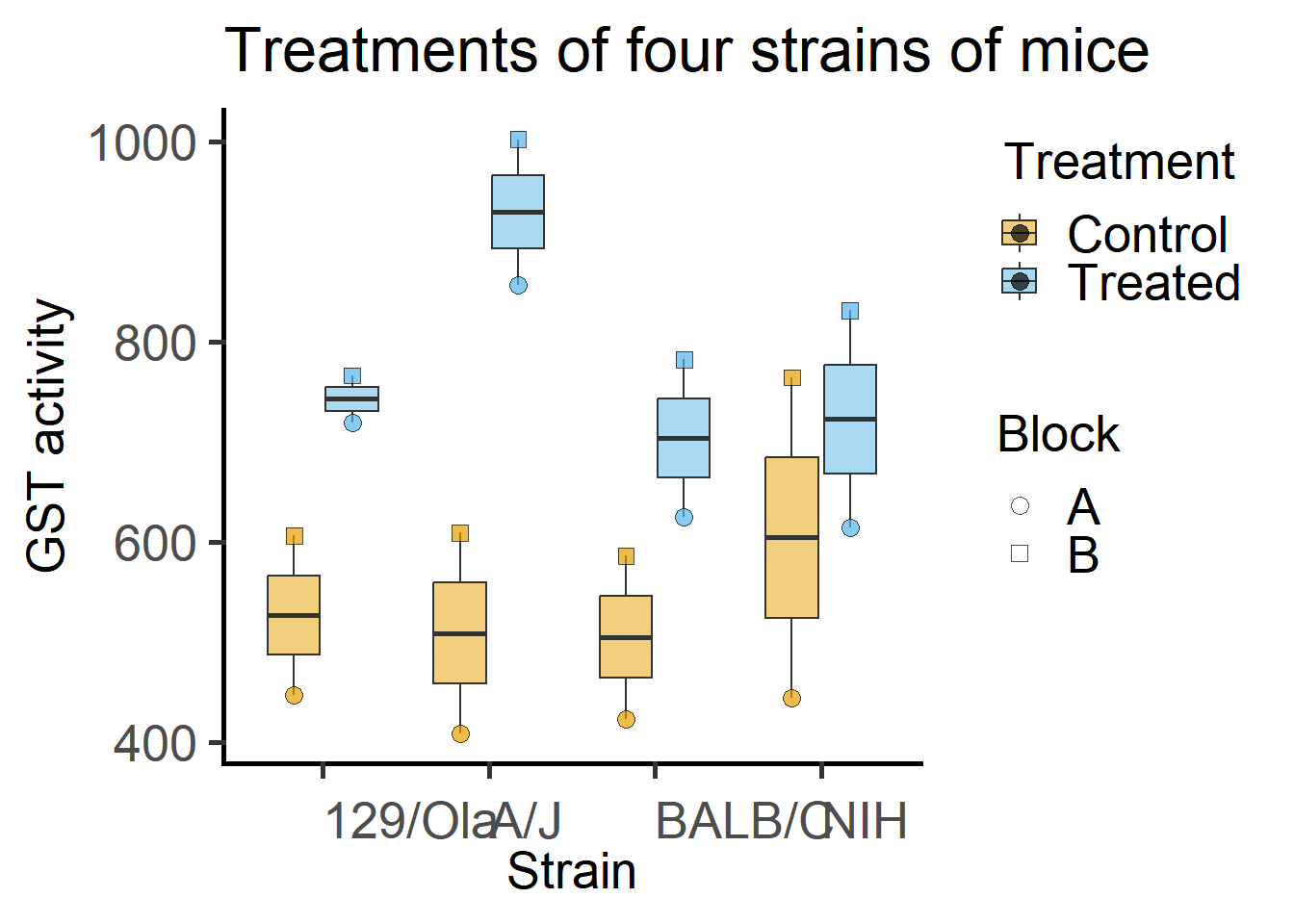

Figure 6.1: Treatment of four strains of mice in block design

By eye-balling these data it appears that Treatment increases GST levels, but that this effect may be lesser in magnitude in the NIH strain.

We can also plot the data for each Block separately.

ggplot(Mice, 
       aes(x = Strain, 
           y = GST))+
  geom_point(aes(fill = Treatment,
                 shape = Treatment),
             alpha = 0.6,
             size = 3,
             position = position_dodge(width = 1))+
  geom_line(aes(group = Strain),
             position = position_dodge2(width = 1))+
  facet_grid("Block")+
  theme_grafify(base_size = 18)+
  scale_fill_grafify()+
  scale_shape_manual(values = 21:22)+
  labs(title = "Plot of each experimental Block",
       x = "Strain", 
       y = "GST activity")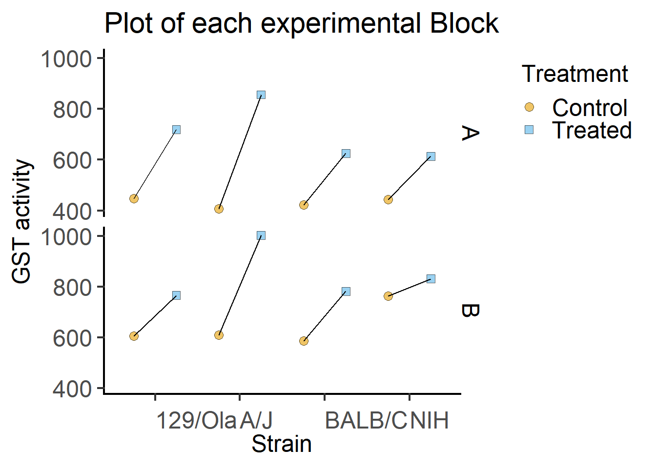

Figure 6.2: Plot of two experimental blocks

6.2 The mixed model for mouse treatments

In this data set, Y = GST activity (the dependent variable) predicted by Strain and Treatment (which are fixed factors), and Exp is the random factor.

Tip

The syntax for lme() is of the Y ~ X + (1|R) style, where Y is the dependent variable, X (one or more) are the fixed factors (the predictors) and (1|R) is the syntax for intercepts of the random factor. The quantitative variable is always on the left of the ~ and predictors on the right.

Micelmer <- lmer(GST ~ Strain*Treatment + # formula for the model
                   (1|Block), #random factor
                 data = Mice) # data table

We can see the details of the model using the summary() call. The model and various details pop-up. The random factor details are provided separately on top. This is similar to the way we read results in Chapter 4.

An important thing to note is that in the section on Random effects which shows that the Std.Dev. of the random factor is greater than the Residual Std.Dev. Note that Std.Dev. of Block is 123.14 and the Residual is 54.38, which suggests that a large portion of \(noise\) was attributed to the random factor. An ordinary ANOVA analyses will likely be less powerful, see below.

The next part listing the number of observations (16) in two groups also looks right.

The first row in the section below gives us the overall Intercept, which by default is the alphabetically first group. (Remember you can use fct_relevel() to change order of groups). Changing the order of groups will not affect the ANOVA result!

The rest of the result shows rows with slopes (coefficients) for all combinations of levels as compared to the overall intercept. As these are linear models, they follow \(y = mx + c + \epsilon\), so each value can be calculated as slope * x + intercept \(\pm\) residual error.

summary(Micelmer) #lmer() model summary

Linear mixed model fit by REML. t-tests use Satterthwaite's method ['lmerModLmerTest']
Formula: GST ~ Strain * Treatment + (1 | Block)
   Data: Mice

REML criterion at convergence: 95.9

Scaled residuals: 
    Min      1Q  Median      3Q     Max 
-1.3603 -0.2462  0.0000  0.2462  1.3603 

Random effects:
 Groups   Name        Variance Std.Dev.
 Block    (Intercept) 15162    123.14  
 Residual              2957     54.38  
Number of obs: 16, groups:  Block, 2

Fixed effects:
                              Estimate Std. Error      df t value Pr(>|t|)   
(Intercept)                    526.500     95.183   1.356   5.531  0.06830 . 
StrainA/J                      -18.000     54.381   7.000  -0.331  0.75033   
StrainBALB/C                   -22.000     54.381   7.000  -0.405  0.69788   
StrainNIH                       77.500     54.381   7.000   1.425  0.19714   
TreatmentTreated               216.000     54.381   7.000   3.972  0.00538 **
StrainA/J:TreatmentTreated     204.500     76.906   7.000   2.659  0.03251 * 
StrainBALB/C:TreatmentTreated  -17.000     76.906   7.000  -0.221  0.83136   
StrainNIH:TreatmentTreated     -97.500     76.906   7.000  -1.268  0.24541   
---
Signif. codes:  0 '***' 0.001 '**' 0.01 '*' 0.05 '.' 0.1 ' ' 1

Correlation of Fixed Effects:
            (Intr) StrA/J StBALB/C StrNIH TrtmnT SA/J:T SBALB/C:
StrainA/J   -0.286                                              
StranBALB/C -0.286  0.500                                       
StrainNIH   -0.286  0.500  0.500                                
TretmntTrtd -0.286  0.500  0.500    0.500                       
StrnA/J:TrT  0.202 -0.707 -0.354   -0.354 -0.707                
StBALB/C:TT  0.202 -0.354 -0.707   -0.354 -0.707  0.500         
StrnNIH:TrT  0.202 -0.354 -0.354   -0.707 -0.707  0.500  0.500  

This model gives us the predicted value of GST based on a mixed linear effects model fit to observed data. The observed GST values will be slightly different, but close enough if our model is good!

6.2.1 Model diagnostics

We can find out how good using model diagnostics with the ggResidpanel package. As for any linear line, the residuals should be randomly and normally distributed without any patterns. The ggResidpanel vignette is here.

resid_panel(Micelmer) #model diagnostics

Figure 6.3: Model diagnostics.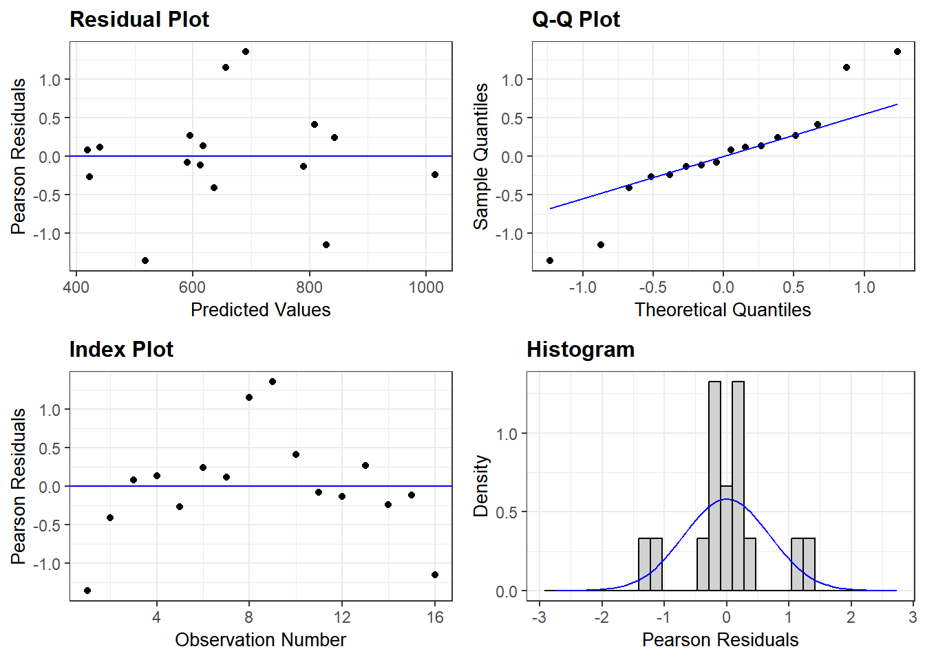

It looks like there are no major concerns with the residuals of this model. SO we can proceed with getting an ANOVA table and post-hoc comparisons.

6.2.2 ANOVA table

We will use the anova() call for the ANOVA table with the F statistic and P values. We will get P values only if lmerTest() is loaded before fitting the model. The default for lme4 package is to only provide F values (because calculating denDf for complex designs is not easy, and P values depend on numDf and denDf but F values only depend on the raw data). Like we discussed in Chapter 4, the F statistic is the ratio of the mean sum of square for each row and the residual variance of the overall model (from the summary() above).

anova(Micelmer, #anova (lmerTest)
      type = "II")  #get type II sum of squares - recommended

Type II Analysis of Variance Table with Satterthwaite's method
                 Sum Sq Mean Sq NumDF DenDF F value    Pr(>F)    
Strain            28613    9538     3     7  3.2252   0.09144 .  
Treatment        227529  227529     1     7 76.9394 5.041e-05 ***
Strain:Treatment  49590   16530     3     7  5.5897   0.02832 *  
---
Signif. codes:  0 '***' 0.001 '**' 0.01 '*' 0.05 '.' 0.1 ' ' 1

The F value is very large for Treatment, and relatively small for the interaction between Treatment and Strain. Strain does not seem to have a large F, but given the small \(signal\) for interaction, we might want to look at what is going on. This suggests that Treatment affects GST outcome, but the Strain of mice does not have an effect on this. The interaction suggests that the effect of Treatment on different Strains may be different.

See Chapter 5 for how to report ANOVA results. Here we would report it for each fixed factor and interaction separately.

6.3 Post-hoc comparisons of treatments

We use emmeans for this as below, which we also used here in Chapter 5. Three different post-hoc comparisons shown below as examples, but post-hoc tests should be ‘planned’ before analysis. The emmeans programme is quite powerful and allows many different options for post-hoc comparisons.

See here and here for advanced ways of setting up comparisons, and changing methods for dDf calculations etc.

6.3.1 Comparisons of Control vs Treatment for each Strain

Use the | operator with factors on each side: it could be read as pairwise comparisons of Treatment levels separately at each level of Strain.

emmeans(Micelmer, 
        pairwise ~ Treatment|Strain, #pairwise comparisons of Treatment at each level of strain
        adjust = "fdr", #adjustment for multiple comparisons
        type = "response") #back-transform (of transformation indicated in lmer() formula)

$emmeans
Strain = 129/Ola:
 Treatment emmean   SE   df lower.CL upper.CL
 Control      526 95.2 1.36   -140.0     1193
 Treated      742 95.2 1.36     76.0     1409

Strain = A/J:
 Treatment emmean   SE   df lower.CL upper.CL
 Control      508 95.2 1.36   -158.0     1175
 Treated      929 95.2 1.36    262.5     1595

Strain = BALB/C:
 Treatment emmean   SE   df lower.CL upper.CL
 Control      504 95.2 1.36   -162.0     1171
 Treated      704 95.2 1.36     37.0     1370

Strain = NIH:
 Treatment emmean   SE   df lower.CL upper.CL
 Control      604 95.2 1.36    -62.5     1270
 Treated      722 95.2 1.36     56.0     1389

Degrees-of-freedom method: kenward-roger 
Confidence level used: 0.95 

$contrasts
Strain = 129/Ola:
 contrast          estimate   SE df t.ratio p.value
 Control - Treated     -216 54.4  7  -3.972  0.0054

Strain = A/J:
 contrast          estimate   SE df t.ratio p.value
 Control - Treated     -420 54.4  7  -7.733  0.0001

Strain = BALB/C:
 contrast          estimate   SE df t.ratio p.value
 Control - Treated     -199 54.4  7  -3.659  0.0081

Strain = NIH:
 contrast          estimate   SE df t.ratio p.value
 Control - Treated     -118 54.4  7  -2.179  0.0657

Degrees-of-freedom method: kenward-roger 

All versus all comparisons are also possible (not advised when there are many levels in each factor) with pairwise ~ Treatment:Strain. Note the use of : as opposed to |.

6.3.2 Comparison of the response of each Strain to the Treatment

Swapping Strain and Treatment gets us pairwise comparison of each level of Strain separately for each level of Treatment.

emmeans(Micelmer, 
        pairwise ~ Strain|Treatment, #pairwise comparisons of Strain
        adjust = "fdr", 
        type = "response")

$emmeans
Treatment = Control:
 Strain  emmean   SE   df lower.CL upper.CL
 129/Ola    526 95.2 1.36   -140.0     1193
 A/J        508 95.2 1.36   -158.0     1175
 BALB/C     504 95.2 1.36   -162.0     1171
 NIH        604 95.2 1.36    -62.5     1270

Treatment = Treated:
 Strain  emmean   SE   df lower.CL upper.CL
 129/Ola    742 95.2 1.36     76.0     1409
 A/J        929 95.2 1.36    262.5     1595
 BALB/C     704 95.2 1.36     37.0     1370
 NIH        722 95.2 1.36     56.0     1389

Degrees-of-freedom method: kenward-roger 
Confidence level used: 0.95 

$contrasts
Treatment = Control:
 contrast             estimate   SE df t.ratio p.value
 (129/Ola) - (A/J)        18.0 54.4  7   0.331  0.9004
 (129/Ola) - (BALB/C)     22.0 54.4  7   0.405  0.9004
 (129/Ola) - NIH         -77.5 54.4  7  -1.425  0.3943
 (A/J) - (BALB/C)          4.0 54.4  7   0.074  0.9434
 (A/J) - NIH             -95.5 54.4  7  -1.756  0.3675
 (BALB/C) - NIH          -99.5 54.4  7  -1.830  0.3675

Treatment = Treated:
 contrast             estimate   SE df t.ratio p.value
 (129/Ola) - (A/J)      -186.5 54.4  7  -3.430  0.0220
 (129/Ola) - (BALB/C)     39.0 54.4  7   0.717  0.7371
 (129/Ola) - NIH          20.0 54.4  7   0.368  0.7371
 (A/J) - (BALB/C)        225.5 54.4  7   4.147  0.0202
 (A/J) - NIH             206.5 54.4  7   3.797  0.0202
 (BALB/C) - NIH          -19.0 54.4  7  -0.349  0.7371

Degrees-of-freedom method: kenward-roger 
P value adjustment: fdr method for 6 tests 

6.3.3 Comparison of the Treatment responses of all strains to A/J strain as an example

To get comparisons to a “control” or “reference” group, use the trt.vs.ctrl specification and set a reference group.

emmeans(Micelmer, 
        trt.vs.ctrl ~ Strain|Treatment, #comparison to a reference control
        ref = 2, #number of reference level (alphabetical by default)
        adjust = "fdr", 
        type = "response")

$emmeans
Treatment = Control:
 Strain  emmean   SE   df lower.CL upper.CL
 129/Ola    526 95.2 1.36   -140.0     1193
 A/J        508 95.2 1.36   -158.0     1175
 BALB/C     504 95.2 1.36   -162.0     1171
 NIH        604 95.2 1.36    -62.5     1270

Treatment = Treated:
 Strain  emmean   SE   df lower.CL upper.CL
 129/Ola    742 95.2 1.36     76.0     1409
 A/J        929 95.2 1.36    262.5     1595
 BALB/C     704 95.2 1.36     37.0     1370
 NIH        722 95.2 1.36     56.0     1389

Degrees-of-freedom method: kenward-roger 
Confidence level used: 0.95 

$contrasts
Treatment = Control:
 contrast          estimate   SE df t.ratio p.value
 (129/Ola) - (A/J)     18.0 54.4  7   0.331  0.9434
 (BALB/C) - (A/J)      -4.0 54.4  7  -0.074  0.9434
 NIH - (A/J)           95.5 54.4  7   1.756  0.3675

Treatment = Treated:
 contrast          estimate   SE df t.ratio p.value
 (129/Ola) - (A/J)   -186.5 54.4  7  -3.430  0.0110
 (BALB/C) - (A/J)    -225.5 54.4  7  -4.147  0.0101
 NIH - (A/J)         -206.5 54.4  7  -3.797  0.0101

Degrees-of-freedom method: kenward-roger 
P value adjustment: fdr method for 3 tests 

6.3.4 Approx Df calculations of mouse treatments

• \(signal\) Df for Strains = 4 – 1 = 3

• \(signal\) Df for Treatment = 2 – 1 = 1

• Interaction Signal = 3 x 1 = 3

• Blocks = 2 – 1 = 1

• Total samples Df = 16 – 1 = 15

• \(noise\) Df = 15 – 3 – 1 – 3 – 1 = 7

Check out tutorial on Df by Ron Dotsch here.

6.4 Ordinary two-way ANOVA

Just as we did here in Chapter 5, I illustrate analyses of these data as an ordinary two-way ANOVA using lm from base R by ignoring the blocking factor. The results are different!

Micelm <- lm(GST ~ Strain*Treatment,  # formula for the model
             data = Mice) # data table

summary(Micelm)  #model summary

Call:
lm(formula = GST ~ Strain * Treatment, data = Mice)

Residuals:
   Min     1Q Median     3Q    Max 
  -160    -80      0     80    160 

Coefficients:
                              Estimate Std. Error t value Pr(>|t|)    
(Intercept)                     526.50      95.18   5.531 0.000553 ***
StrainA/J                       -18.00     134.61  -0.134 0.896926    
StrainBALB/C                    -22.00     134.61  -0.163 0.874228    
StrainNIH                        77.50     134.61   0.576 0.580620    
TreatmentTreated                216.00     134.61   1.605 0.147239    
StrainA/J:TreatmentTreated      204.50     190.37   1.074 0.314042    
StrainBALB/C:TreatmentTreated   -17.00     190.37  -0.089 0.931037    
StrainNIH:TreatmentTreated      -97.50     190.37  -0.512 0.622368    
---
Signif. codes:  0 '***' 0.001 '**' 0.01 '*' 0.05 '.' 0.1 ' ' 1

Residual standard error: 134.6 on 8 degrees of freedom
Multiple R-squared:  0.6784,    Adjusted R-squared:  0.3969 
F-statistic:  2.41 on 7 and 8 DF,  p-value: 0.1205

As we expected, the residual error is large (134.6) compared to the mixed effects model above (where it was 54.38).

I use the Anova call from the car package [2] (as the anova call only gives type I ANOVAs, it cannot be used here in a two-way ANOVA with interaction).

car::Anova(Micelm,               #Anova call from "car" package
           type = "II",          #this is also the default
           test.statistic = "F") #to get F values

Warning in printHypothesis(L, rhs, names(b)): one or more coefficients in the hypothesis include
     arithmetic operators in their names;
  the printed representation of the hypothesis will be omitted

Warning in printHypothesis(L, rhs, names(b)): one or more coefficients in the hypothesis include
     arithmetic operators in their names;
  the printed representation of the hypothesis will be omitted

Warning in printHypothesis(L, rhs, names(b)): one or more coefficients in the hypothesis include
     arithmetic operators in their names;
  the printed representation of the hypothesis will be omitted

Anova Table (Type II tests)

Response: GST
                 Sum Sq Df F value  Pr(>F)   
Strain            28613  3  0.5264 0.67640   
Treatment        227529  1 12.5570 0.00758 **
Strain:Treatment  49591  3  0.9123 0.47705   
Residuals        144957  8                   
---
Signif. codes:  0 '***' 0.001 '**' 0.01 '*' 0.05 '.' 0.1 ' ' 1

In this case, the result is quite different from that obtained with mixed effects model above!

emmeans(Micelm, 
        pairwise ~ Treatment|Strain, #pairwise comparisons of Treatments
        adjust = "fdr", 
        type = "response")

$emmeans
Strain = 129/Ola:
 Treatment emmean   SE df lower.CL upper.CL
 Control      526 95.2  8      307      746
 Treated      742 95.2  8      523      962

Strain = A/J:
 Treatment emmean   SE df lower.CL upper.CL
 Control      508 95.2  8      289      728
 Treated      929 95.2  8      710     1148

Strain = BALB/C:
 Treatment emmean   SE df lower.CL upper.CL
 Control      504 95.2  8      285      724
 Treated      704 95.2  8      484      923

Strain = NIH:
 Treatment emmean   SE df lower.CL upper.CL
 Control      604 95.2  8      385      823
 Treated      722 95.2  8      503      942

Confidence level used: 0.95 

$contrasts
Strain = 129/Ola:
 contrast          estimate  SE df t.ratio p.value
 Control - Treated     -216 135  8  -1.605  0.1472

Strain = A/J:
 contrast          estimate  SE df t.ratio p.value
 Control - Treated     -420 135  8  -3.124  0.0141

Strain = BALB/C:
 contrast          estimate  SE df t.ratio p.value
 Control - Treated     -199 135  8  -1.478  0.1776

Strain = NIH:
 contrast          estimate  SE df t.ratio p.value
 Control - Treated     -118 135  8  -0.880  0.4044

Note that in these analyses only one strain (A/J) shows a significant effects of Treatment on GST.

The increased power in being able to detect small differences in these variables was possible because the experiment was designed as randomised-blocks and analysed using mixed linear effects.

6.5 Two-way ANOVA with grafify

The same functions in grafify can do one or multi-way ANOVAs as linear models (simple_model or mixed_model). Please see further details on the grafify vignette website for ordinary ANOVA and mixed models.

#fit a model
graf_2w_model <- mixed_model(data = Mice,
                             Y_value = "GST",
                             Fixed_Factor = c("Strain",
                                              "Treatment"),
                             Random_Factor = "Block")

#QQ plot of model residuals
plot_qqmodel(Model = graf_2w_model)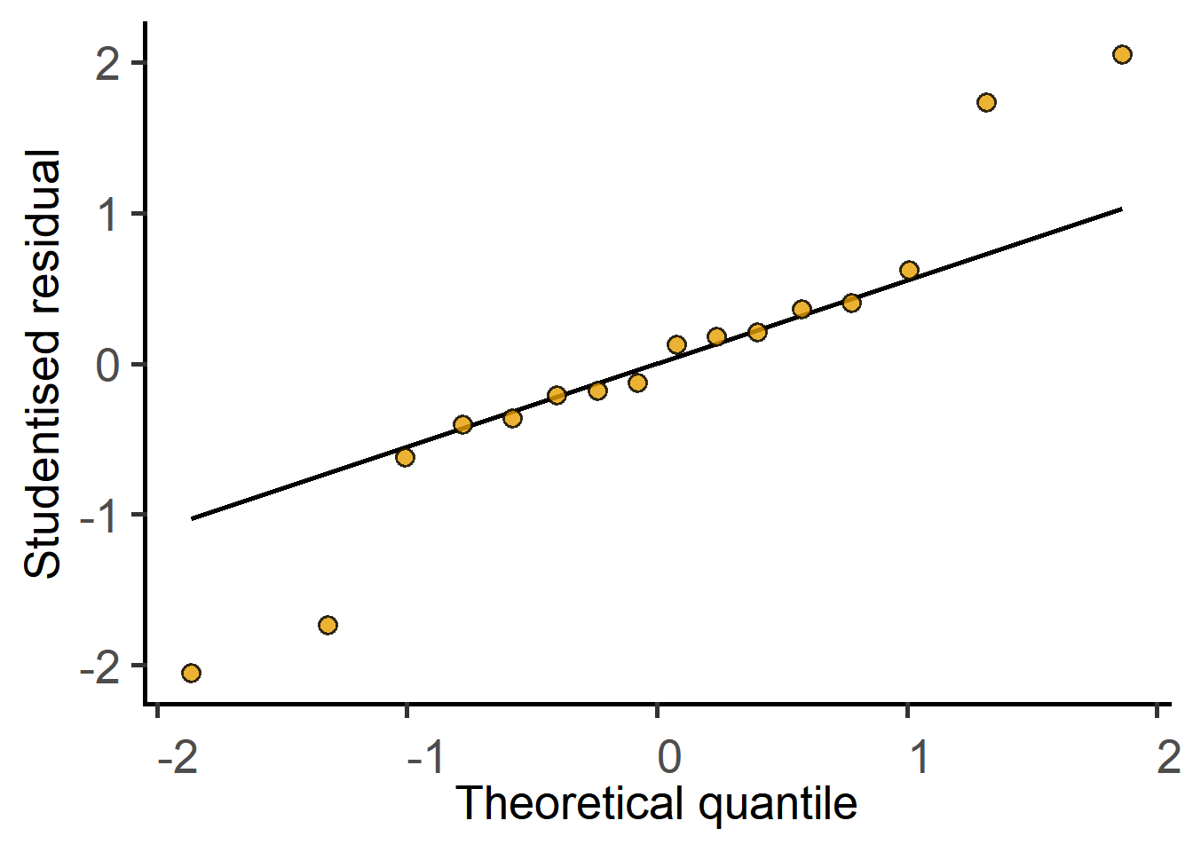

Two-way ANOVA with grafify

#ANOVA table
mixed_anova(data = Mice,
            Y_value = "GST",
            Fixed_Factor = c("Strain",
                             "Treatment"),
            Random_Factor = "Block")

Type II Analysis of Variance Table with Kenward-Roger's method
                 Sum Sq Mean Sq NumDF DenDF F value    Pr(>F)    
Strain            28613    9538     3     7  3.2252   0.09144 .  
Treatment        227529  227529     1     7 76.9394 5.041e-05 ***
Strain:Treatment  49591   16530     3     7  5.5897   0.02832 *  
---
Signif. codes:  0 '***' 0.001 '**' 0.01 '*' 0.05 '.' 0.1 ' ' 1

#posthoc comparisons at each level
posthoc_Levelwise(Model = graf_2w_model,
                  Fixed_Factor = c("Treatment",
                                   "Strain"))

$emmeans
Strain = 129/Ola:
 Treatment emmean   SE   df lower.CL upper.CL
 Control      526 95.2 1.36   -140.0     1193
 Treated      742 95.2 1.36     76.0     1409

Strain = A/J:
 Treatment emmean   SE   df lower.CL upper.CL
 Control      508 95.2 1.36   -158.0     1175
 Treated      929 95.2 1.36    262.5     1595

Strain = BALB/C:
 Treatment emmean   SE   df lower.CL upper.CL
 Control      504 95.2 1.36   -162.0     1171
 Treated      704 95.2 1.36     37.0     1370

Strain = NIH:
 Treatment emmean   SE   df lower.CL upper.CL
 Control      604 95.2 1.36    -62.5     1270
 Treated      722 95.2 1.36     56.0     1389

Degrees-of-freedom method: kenward-roger 
Confidence level used: 0.95 

$contrasts
Strain = 129/Ola:
 contrast          estimate   SE df t.ratio p.value
 Control - Treated     -216 54.4  7  -3.972  0.0054

Strain = A/J:
 contrast          estimate   SE df t.ratio p.value
 Control - Treated     -420 54.4  7  -7.733  0.0001

Strain = BALB/C:
 contrast          estimate   SE df t.ratio p.value
 Control - Treated     -199 54.4  7  -3.659  0.0081

Strain = NIH:
 contrast          estimate   SE df t.ratio p.value
 Control - Treated     -118 54.4  7  -2.179  0.0657

Degrees-of-freedom method: kenward-roger 

[1]

M.F.W. Festing, Randomized Block Experimental Designs Can Increase the Power and Reproducibility of Laboratory Animal Experiments, ILAR Journal 55 (2014) 472–476. https://doi.org/10.1093/ilar/ilu045.

[2]

J. Fox, S. Weisberg, B. Price, Car: Companion to applied regression, 2020. https://CRAN.R-project.org/package=car.