2 Getting started
2.1 Installation steps
Follow the steps in this order.
R is freely available from The Comprehensive R Archive Network (CRAN). Go to the CRAN website and use the links at the top for your OS (operating system, e.g., Windows or MacOS or Linux) to download and install R. Use default options during installation.
RStudio Desktop is a free IDE (integrated development environment) that makes it very easy to use R that we installed in step 1. Go to the RStudio website and install their free RStudio Desktop version for your OS. Use default options during installation. Note that RStudio was recently renamed “Posit”, but nothing has changed for users. I still call it RStudio.
Open RStudio and familiarise yourself with the four windows or “panes”. You could start by watching these short videos (will likely need Imperial login to access the Sharepoint site), the first one Getting started with R - intro session 1 explains the installation process.
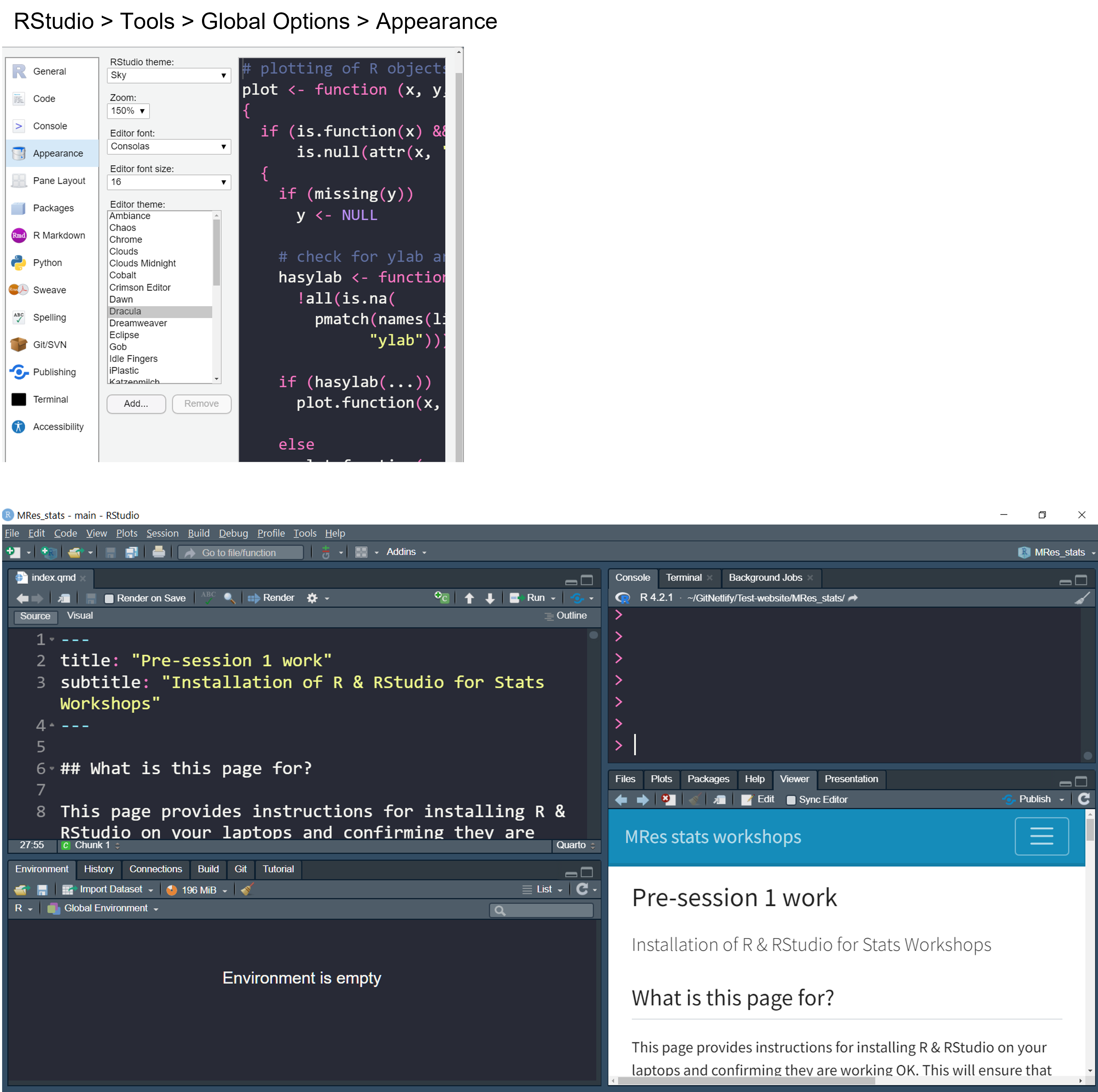
My RStudio looks like this (settings on top and appearance below), but you can use settings you prefer!
- For code in this book, we will need several plotting and statistics packages. To install them, copy the code below to your ‘console’ and hit ENTER to run it. It could take several minutes to download and install all required packages. Note that R is case sensitive (
knitris not the same asKnitr,KNITRor other variants).
install.packages(c("rmarkdown", "knitr", "readr", "readxl", "grafify", "ggResidpanel"), dependencies = TRUE)
The above code will download and install various packages, and could take some time depending on your device and internet connection.
Depending on your OS and other settings, during the installation process you might be asked questions, for example:
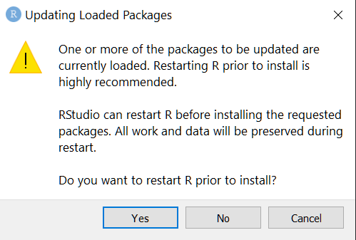
For this question, it is good to say “Yes” once; if it asks the same again, say “No” and proceed.
Another question could be:
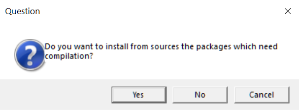
Say “No” and proceed (building from source needs more software and can be much more time-consuming).
2.1.1 What if there are errors?
The easiest thing to do if there are errors is to copy the text of the error and do a Google search. Almost all errors have been experienced by other users and there may be help online to resolve them.
2.2 The basic R operators
Let’s first look at the common operators in R. You can type the code on your console as you go along. Remember that R is sensitive to case (i.e., Alpha is not the same as alpha).
<-assign operator (you can also use=) is used to assign values and create objects in R. It is the less-than sign and hyphen without space. Shortcut:Alt&-together.
Create your first objects Alpha and five as below. They will then appear in your Environment pane.
#an object with an alphabet
Alpha <- "A"
#an object with one number
five <- 5#comment on lines of code. Starting code with#will prevent the line from being executed, and is therefore used to add comments. For example, typing5*6on the console will give you the result (30), but# 5*6will not work because R thinks that’s a comment.*,/,+,-,^, and()are common math operators.
# a comment
7*3 #three times seven
[1] 21#7*3 is also a comment
#mathematical operation on an object
five * 5 [1] 25#this will fail try it without the #
#Alpha * 5= equal symbol is used to assign an argument of a function.
In R, the function head can be used to see the top 6 rows of a table. By adding ad additional argument n, we can view a select number of rows.
Let’s use this function the table cars.
head(cars) #shows top 6 rows by default speed dist
1 4 2
2 4 10
3 7 4
4 7 22
5 8 16
6 9 10#with a value to an argument for head
head(cars, n = 3) #show first 3 rows speed dist
1 4 2
2 4 10
3 7 4#see the table cars
View(cars) #the table will open in a new tab$dollar operator is used to look up columns in a table.
We can use it to view the columns in the cars table.
#pick the speed column from cars table
cars$speed
[1] 4 4 7 7 8 9 10 10 10 11 11 12 12 12 12 13 13 13 13 14 14 14 14 15 15
[26] 15 16 16 17 17 17 18 18 18 18 19 19 19 20 20 20 20 20 22 23 24 24 24 24 25#mathematical operation on the column
cars$speed + 10 [1] 14 14 17 17 18 19 20 20 20 21 21 22 22 22 22 23 23 23 23 24 24 24 24 25 25
[26] 25 26 26 27 27 27 28 28 28 28 29 29 29 30 30 30 30 30 32 33 34 34 34 34 35[]square brackets have a special meaning, and are typically used for sub-setting data frames (i.e., only picking rows in the table that match a criterion).==(equal to),!=(not equal to),>=(equal to or greater than) or=<(equal to or less than) are logic operators::double colon operator is used to invoke a specificfunctionfrom apackage.
Examples of these operators can be found on the Stats Workshop Session 1 page (link to website above).
2.3 Checking your installation
Check that everything has gone OK by loading one of the packages we installed, and using it to plot a graph. To save memory, R does not load all available packages - the user must invoke them by using the command library, and then use functions in the package.
This is a two-step process.
- First copy the following line to your console and hit ENTER (this will make the
grafifypackage available to use). It will only work if your installation went OK!
library(grafify)
- Next, copy this line to your console and hit ENTER. It should produce a graph using the
grafifypackage.
plot_scatterbox(data_t_pdiff, Condition, Mass)
If all went OK, a graph with scattered symbols with box and whiskers should appear in the Plots pane.
Loading required package: ggplot2Warning in check_dep_version(): ABI version mismatch:
lme4 was built with Matrix ABI version 1
Current Matrix ABI version is 2
Please re-install lme4 from source or restore original 'Matrix' package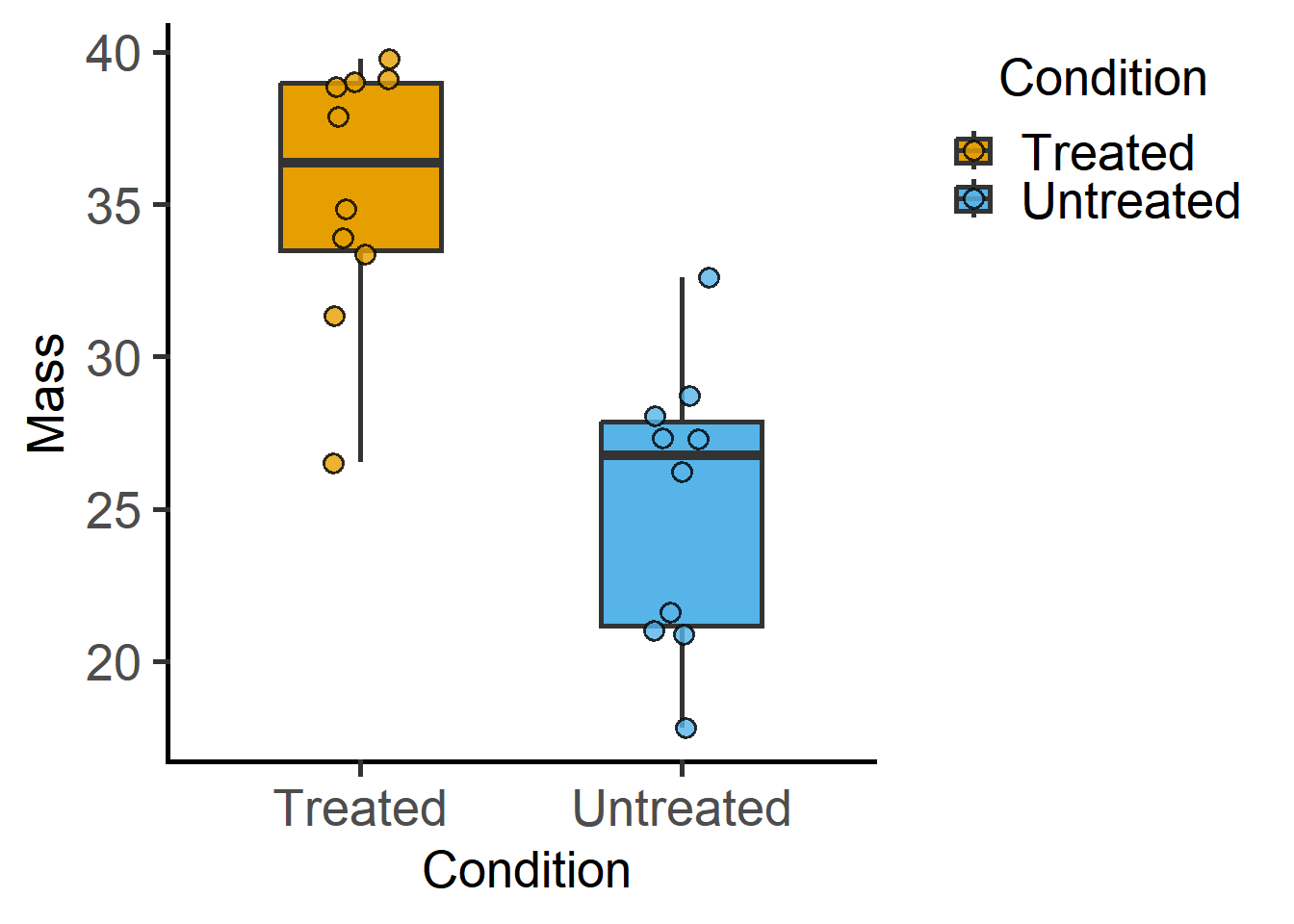
In the function above, we used a data table from the grafify package and used the function plot_scatterbox. First, let’s look at the data table, or more commonly called a data frame in R.
#View function opens the table in the source pane
View(data_t_pdiff)

#names of columns
names(data_t_pdiff)
[1] "Subject" "Condition" "Mass" #structure of the table
str(data_t_pdiff)'data.frame': 20 obs. of 3 variables:
$ Subject : Factor w/ 10 levels "A","B","C","D",..: 1 1 2 2 3 3 4 4 5 5 ...
$ Condition: Factor w/ 2 levels "Treated","Untreated": 2 1 2 1 2 1 2 1 2 1 ...
$ Mass : num 20.9 33.4 21 33.9 28.7 ...You now see that the table has 3 columns, Subject (an ID of each mouse used in the study), Condition (whether a mouse was Treated or Untreated with a drug) and Mass (its body weight in grams).
When we plotted the graph above, we used the first three arguments in their default order. We can be more explicit as below.
plot_scatterbox(data = data_t_pdiff,    #name of data frame
                xcol = Condition,       #column to plot on X axis
                ycol = Mass)            #column to plot on Y axis
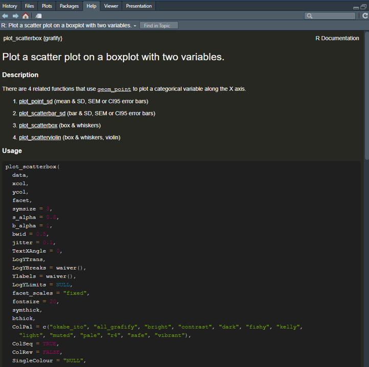
No one can remember the arguments, let alone their order for all the functions in R. But do not worry, help is nearby. Adding a ? before the name of the function gives you usage details in the Help pane.
?plot_scatterbox()starting httpd help server ... doneThis is how help looks on my Rstudio. As you can see, there are many arguments to tweak the graph, most of which have sensible defaults. We will rarely need to assign a value to all of them, but it’s good to know what can be changed in this graph.
Lastly, you can use :: after the name of a package to find all the functions available in it. Try it with grafify:: and you should be able to scroll through a list of data frames and functions in this package. When first starting out in R for statistics, use a small dataset that you have previously analysed (e.g. in Prism). When you first start, ensure that your data table is ‘ready’ to be plotted and you’ve performed any necessary data wrangling, calculations or transformations already. Tips on doing this are in the Appendix. This way you can get to the analysis itself with fewer errors, and focus on familiarising the output from R and compare it to the output from other software.
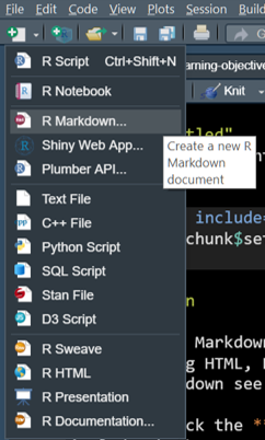
2.4 R Markdown
Once you start, one thing you want to know how to do is how to save your work. For all your analyses, I highly recommend that you write all code, results, analysis, graphs etc. in R Markdown.
An RMarkdown file has a .Rmd extension and contains R code that can be run and executed by anyone who you share it with. This is great for reproducibility and sharing your results. You can also have rich text such as bold, italics, superscript, subscript etc., in your outputs (further details in the Appendix). This website/book is written entirely using RMarkdown in RStudio!
The knitr package ‘knits’ .Rmd files into HTML files that open in a browser. Other output formats are also possible (e.g., Word or PDF files), but I do not recommend them. Further resources are listed in the Appendix.
Read more here about how to make nice RMarkdown outputs.
2.5 grafify package
The grafify package simplifies R for plotting graphs, performing ANOVAs and post-hoc comparisons. How to use grafify for analyses and graphs is shown in Chapter 9. More detailed instructions on using grafify are at the vignettes website.
grafify can plot the following 19 common types of graphs with fewer lines of code, and provides 9 colour blind-friendly colour schemes.
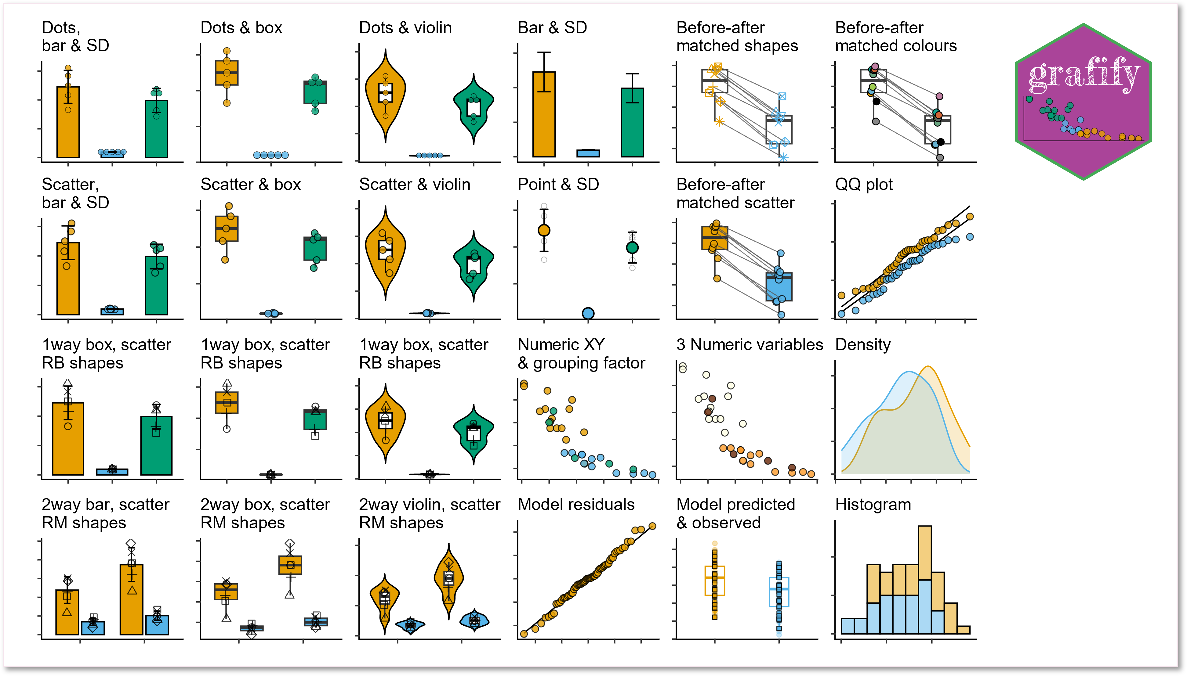
grafify also contains datasets used in this document. Note that the code used in this document shows native usage of R packages that grafify relies on (e.g. ggplot2, lmerTest, emmeans).
Download and install grafify from CRAN or GitHub.
install.packages("grafify")If you use grafify, please cite
Shenoy, A. R. (2021) grafify: an R package for easy graphs, ANOVAs and post-hoc comparisons. Zenodo. http://doi.org/10.5281/zenodo.5136508
Latest DOI for all versions: ![]()
2.6 Further resources
Here are some selected resources to introduce you to R/RStudio. There are many others as you can find for yourself on the web.
Here are instructions for installing R and simple exercises.
Watch this YouTube Video.
Use this excellent RLadies BasicBasics tutorial.
This can be too much to start with at one go. Why not pace yourself with this tutorial from Software Carpentry at Imperial College? Doing a little bit every so often is the best way to get used to R.
If you are a student/staff at Imperial College, register for access to LinkedIn Learning using your College ID and check out the Learning R and Data Wrangling courses by Barton Poulson.
Code can often fail - do not let this disappoint you. It is because of this that there are dedicated websites for Q&A – use them! When searching online, use Stackexchange or Stackoverflow. I learnt a lot of R by reading Q&A on Stack!
When using R, if you forget a function, using
?Name of Functionwill take you to the help page in the Viewer panel. R is case-sensitive, sostatsis not the same asSTATS!Note that in almost all cases, data tables for analysis in R should be in “long format”. It’s easy to change formats from wide to long in R, as shown in the Appendix.
2.7 Further help
The Appendix has sections on help with R packages necessary to do the tests in this document and plot similar looking graphs.