| X | Experiment | Genotype | Death |
|---|---|---|---|
| 1 | Exp_1 | WT | 25.012 |
| 2 | Exp_1 | mfg | 1.825 |
| 3 | Exp_1 | yfg | 14.295 |
| 4 | Exp_2 | WT | 16.543 |
| 5 | Exp_2 | mfg | 2.131 |
| 6 | Exp_2 | yfg | 23.749 |
| 7 | Exp_3 | WT | 31.126 |
| 8 | Exp_3 | mfg | 1.917 |
| 9 | Exp_3 | yfg | 21.999 |
| 10 | Exp_4 | WT | 21.596 |
| 11 | Exp_4 | mfg | 1.873 |
| 12 | Exp_4 | yfg | 16.445 |
| 13 | Exp_5 | WT | 28.353 |
| 14 | Exp_5 | mfg | 1.956 |
| 15 | Exp_5 | yfg | 22.648 |
5 One-way ANOVA
5.1 Host cell death by three strains of bacteria
These are data from in vitro experiments of death of host cells induced upon infection by three strains of E.coli. Side-by-side experiments were performed 5 times in “blocks” and “Experiment” is a random factor and bacterial “Genotype” is the fixed factor (with three levels, WT, mfg and yfg).
Before proceeding with analysis of your own data, ensure that your data table is in the correct format and categorical variables are encoded as factors and not numbers. Here are the packages needed for these analyses.
5.1.1 Data plots
ggplot(Bact,
       aes(x = Genotype,
           y = Death))+
  geom_boxplot(aes(fill = Genotype),
               width = 0.3,
               alpha = 0.4)+
  geom_point(size = 3.5,
             alpha = 0.9,
             shape = 21,
             aes(fill = Genotype))+
  labs(title = "Cell death during infection",
       x = "Bacterial strain",
       y = "Cell death (%)")+
  theme_grafify()+
  scale_fill_grafify()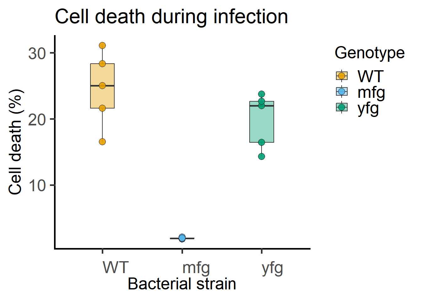
The above data can also be plotted where shape of symbols matches the level of the random factor Experiment.
ggplot(Bact,
       aes(x = Genotype,
           y = Death))+
  geom_boxplot(aes(fill = Genotype),
               width = 0.3,
               alpha = 0.5)+
  geom_point(size = 3.5,
             alpha = 0.9,
             position = position_jitter(width = 0.1),
             aes(fill = Genotype,
                 shape = Experiment))+
  labs(title = "Cell death during infection",
       x = "Bacterial strain",
       y = "Cell death (%)")+
  theme_grafify()+
  scale_fill_grafify()+
  scale_colour_grafify()+
  scale_shape_manual(values = 21:26)+
  guides(fill = guide_legend(override.aes = list(shape = 21)))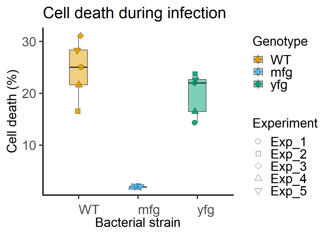
The above graph can be plotted in grafify with fewer lines of code as follows.
library(grafify)
plot_3d_scatterbox(data = Bact,          #data
                   xcol = Genotype,      #X variable
                   ycol = Death,         #Y variable
                   shapes = Experiment)  #blocking variable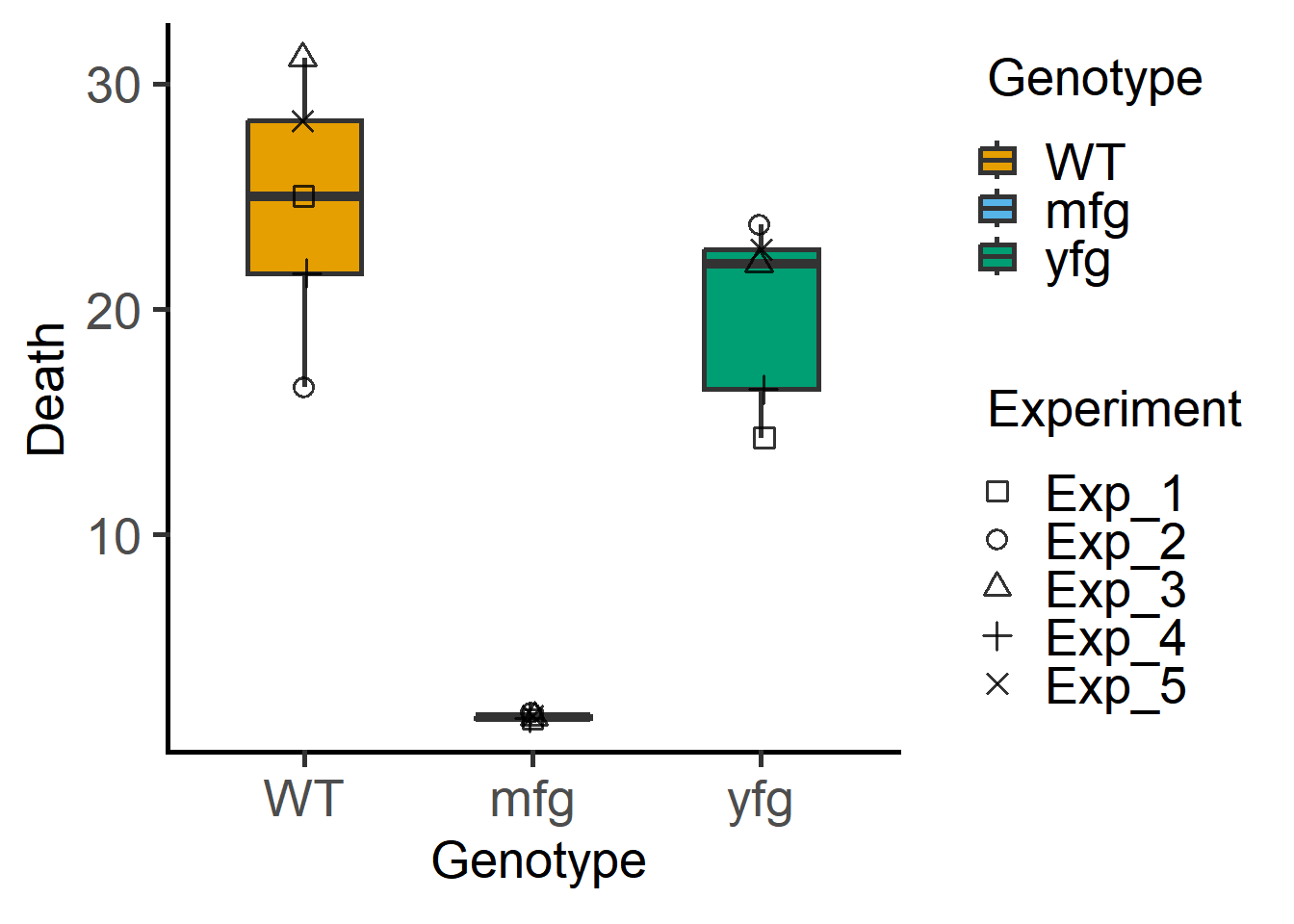
Look at how multiple experiments look, by plotting each one separately. As you can see, the trends between the Genotypes across experiments is the same. The mfg strain has triggered less cell death in all Experiments.
ggplot(Bact,
       aes(x = Genotype,
           y = Death))+
  geom_point(size = 3.5,
             alpha = 0.9,
             shape = 21,
             aes(fill = Genotype))+
  geom_line(aes(group = Experiment))+
  theme_grafify()+
  labs(title = "Cell death during infection",
       x = "Bacterial strain",
       y = "Cell death (%)")+
  scale_fill_grafify()+
  theme(legend.position = "NULL")+
  facet_wrap("Experiment",
             scale = "free")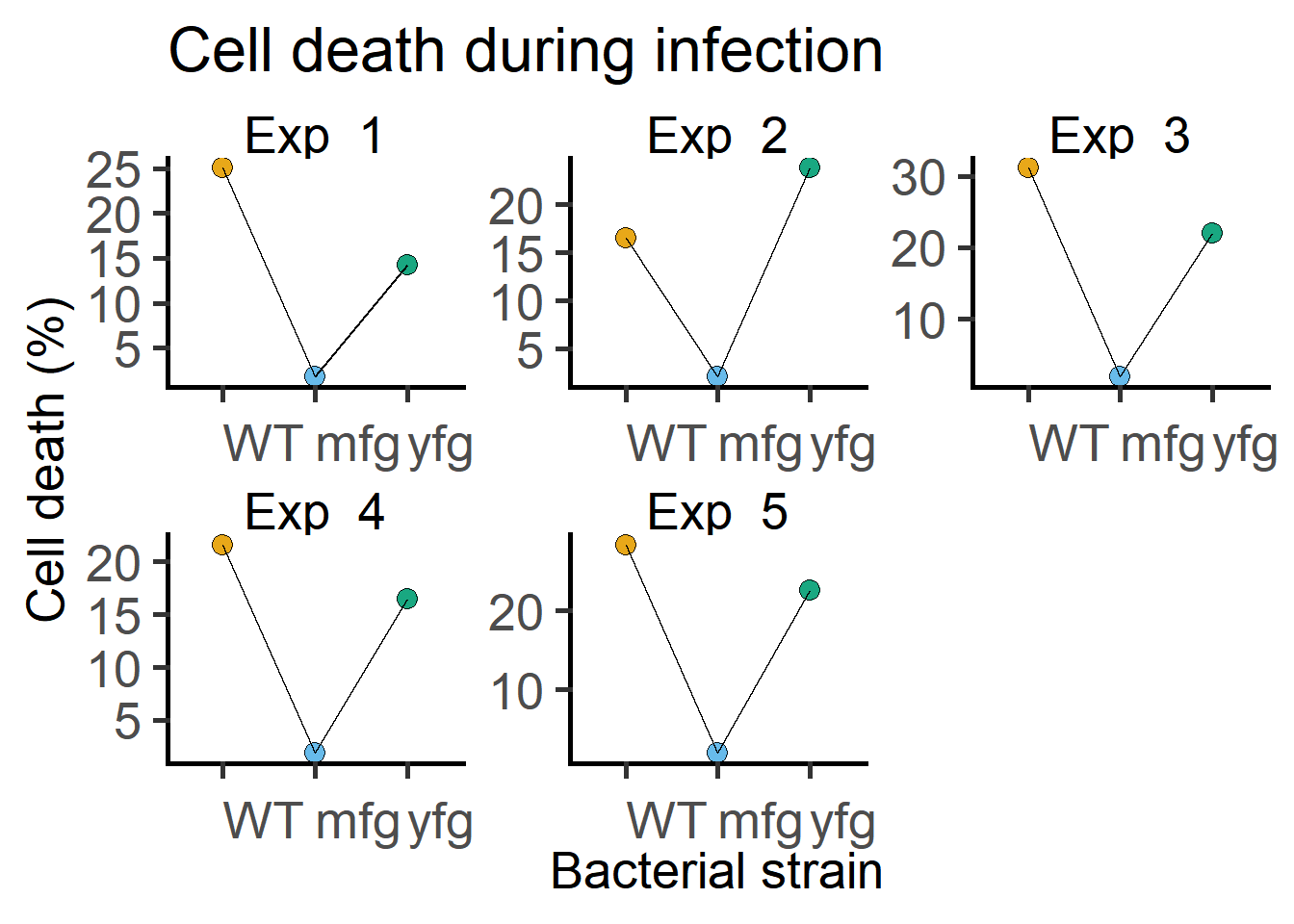
5.2 Data transformation
As these are values of percentage cell death, and some values are very close to 0, it would be acceptable to convert percentages into probabilities (by dividing by 100) and using logit-transformation. This is only possible if there are no values below 0 or negative values. The logit function is available in the bootpackage. Logit is log-odds transformation (i.e. \(log (\frac{p}{1-p})\)), and if done in the formula for lmer and emmeans, it is easier to back-transform them to raw values. This way you will get the mean and SDs etc. on the Death units rather than log-odds scale.
This transformation could improve the model residuals, which we can check with a QQ plot of residuals.
Caution
In ANOVAs (and also Student’s t test), model residuals should be approximately normally distributed. So it is important to plot and inspect them after we fit a linear model, rather than distributions of the data.
5.3 One-way mixed model analysis
We will use lme4 to check whether the fixed factor Genotype has an impact on the dependent variable Death across Experiments (which is a random factor).
It is good-practice to check that factors are coded correctly in the data table using the str() call to ensure that factors and numerical variables are correctly coded in the columns of the table.
#check that Genotype & Experiment are coded as factors
str(Bact)
'data.frame': 15 obs. of 4 variables:
$ X : int 1 2 3 4 5 6 7 8 9 10 ...
$ Experiment: Factor w/ 5 levels "Exp_1","Exp_2",..: 1 1 1 2 2 2 3 3 3 4 ...
$ Genotype : Factor w/ 3 levels "WT","mfg","yfg": 1 2 3 1 2 3 1 2 3 1 ...
$ Death : num 25.01 1.82 14.29 16.54 2.13 ...Mixed models allows us to apportion SD across experiments separately using “Experiment” as a random factor. We allow each experiment to have it’s own baseline by allowing each WT (the first level among Genotypes) to have their own intercepts on the Y axis (i.e. Cell death), and the difference from this intercept (recall that this is the slope) is calculated for the all combinations of levels. The slopes do look consistent across Experiments (based on roughly parallel lines) in the plot in Figure .
5.3.1 ANOVA model
Here, Death (quantitative dependent variable) is the Y variable, and Genotype (fixed factor), with three levels we are interested in comparing, is the X predictor. Experiment is the random factor (also called blocking factor).
Tip
The syntax for lmer() is of the Y ~ X + (1|R) style, where Y is the dependent variable, X (one or more) are the fixed factors (the predictors) and (1|R) is the syntax to allow random factor intercepts. The quantitative variable is always on the left of the ~ (tilde) and predictors on the right.
In this example, I am converting the percentages in the data table into logit in the lmer formula itself. I first divide cell death percentages by 100 and then use the logit() call from the boot package (logit can only be used for values between 0 and 1).
library(boot) #for logit call

Bactlmer <- lmer(logit(Death/100) ~ Genotype + # Y ~ X formula for fixed factor
                   (1|Experiment), #random intercepts for Experiment
                 data=Bact) #data table
summary(Bactlmer)
Linear mixed model fit by REML. t-tests use Satterthwaite's method ['lmerModLmerTest']
Formula: logit(Death/100) ~ Genotype + (1 | Experiment)
Data: Bact
REML criterion at convergence: 5.4
Scaled residuals:
Min 1Q Median 3Q Max
-1.90879 -0.41370 0.03938 0.67946 1.41703
Random effects:
Groups Name Variance Std.Dev.
Experiment (Intercept) 1.303e-18 1.141e-09
Residual 6.141e-02 2.478e-01
Number of obs: 15, groups: Experiment, 5
Fixed effects:
Estimate Std. Error df t value Pr(>|t|)
(Intercept) -1.1454 0.1108 12.0000 -10.335 2.50e-07 ***
Genotypemfg -2.7787 0.1567 12.0000 -17.730 5.67e-10 ***
Genotypeyfg -0.2700 0.1567 12.0000 -1.723 0.111
---
Signif. codes: 0 '***' 0.001 '**' 0.01 '*' 0.05 '.' 0.1 ' ' 1
Correlation of Fixed Effects:
(Intr) Gntypm
Genotypemfg -0.707
Genotypeyfg -0.707 0.500
optimizer (nloptwrap) convergence code: 0 (OK)
boundary (singular) fit: see help('isSingular')5.3.2 ANOVA summary
The
summary()gives us details for the \(y=mx+c\pm error\) equation with an overall intercept (taken as the first level in Genotype, WT) and slopes and SE for each predictor on the X axis. The section on top is about the Random Factor (Experimentin these data), and section below gives details on the levels within the Fixed factors (Genotype).The first thing to note is that it has fit using REML (default, preferred); only change to
REML = FALSEif fitting multiple models to compare.The scaled residuals should have a median around 0.
The Random Effects section has important information. Here we see that the
Experimentas random factor has a very low Std.Dev. of1.141e-09, which suggests that an ordinary ANOVA is likely to give us very similar results.The Residual Std.Dev. is
2.478e-01, which is much higher than the Std.Dev. associated with the random factorExperiment.It is also good to confirm the hierarchy in the data: 15 observations in 5 Experiments.
The section on Fixed effects gives the intercept (by default alphabetically the first level within the factor unless levels are reordered), and key information, such as its Std.Error, degrees of freedom (df),
tstatistic and the P value.Pr(>|t|)means the probability for a t value at least a large as the absolute value (recall that the distribution is symmetric with +ve and -ve values in the tail, therefore the notation for absolute value).The standard * coding for significance is listed next.
At the bottom is the correlation matrix between the levels of the fixed factor.
We can now get the ANOVA table using the model.
anova(Bactlmer,
      type="II") #get type II sum of squares
Type II Analysis of Variance Table with Satterthwaite's method
Sum Sq Mean Sq NumDF DenDF F value Pr(>F)
Genotype 23.48 11.74 2 12 191.18 7.938e-10 ***
---
Signif. codes: 0 '***' 0.001 '**' 0.01 '*' 0.05 '.' 0.1 ' ' 1Also see this for discussion on the ANOVA table in Chapter 4.
In this result, the F value is rather large (191.8) and the chance of getting a value at least as extreme is rather low (
7.9 x 10⁻¹⁰)!Sum Sq divided by the NumDf is the Mean Sq. Mean Sq. divided by the residual variance (
6.141e-02from thesummary()) gives us the F value. See section below on Df calculations.Be careful with
anova()call from basestatspackage in R, where just typing type III will NOT not give the correct output unless columns of factors in the data table are adjusted first withoptions(contrasts=c("contr.sum", "contr.poly")).The discussion on Type I, Type II and Type III sum of squares is beyond the scope of our workshop. The recommendation in the R community is to use Type II by explicitly calling it as below.
5.3.3 Reporting the ANOVA result
The technical way of reporting the result of an ANOVA is to include the F value, both degrees of freedom and the P value.
Here we would say, the result of a one-way ANOVA using linear mixed effects was as follows: F(2, 12) = 191.18; P = 7.938e-10.
Giving details this way gives a more clearer idea of how large the \(signal/noise\) was based on the total number of samples and groups, and the associated P value. The F value and Dfs suggest that this result is suggests a “major” effect of Genotype on cell death.
5.3.4 Model diagnostics
Was the above model a good fit for the data? Here I use the ggResidpanel package for model diagnostics. The ggResidpanel vignette is here.
There should be no visible “patterns” in the Residual Plot and Index Plot. Here we see higher variance as we go left to right on the X axis in the Residual Plot.
In the QQ plot, the theoretical values – i.e. those predicted by the linear equation of our ANOVA model, and sample values (observed data) should lie as close to the line as possible. If the fit is good, the values predicted by the equation will be the same as the observed values.
The histogram of the residuals from the linear fit should have a close to normal distribution. Residuals are unlikely to be normally distributed if points on the QQ Plot are away from the line.
resid_panel(Bactlmer) #model diagnostics: residuals plot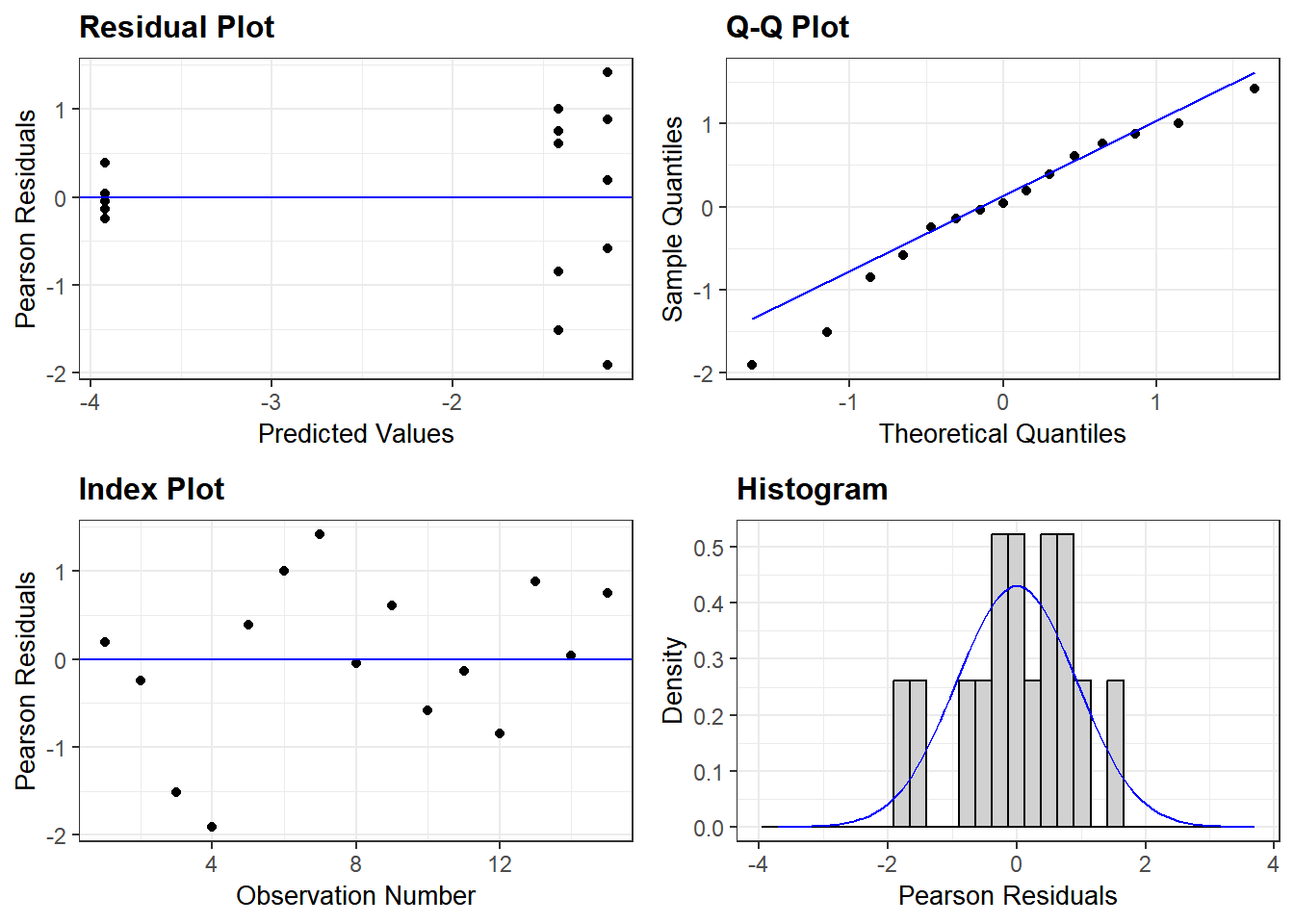
5.3.5 Normality of model residuals
Here is the code for Shapiro-Wilk test on the residuals from the above model.
shapiro.test(resid(Bactlmer)) #resid() calculates residuals & passes on to the test
    Shapiro-Wilk normality test

data:  resid(Bactlmer)
W = 0.96367, p-value = 0.7558
The Shapiro-Wilk test only tells us whether there is support to reject the null hypothesis that data are normally distributed. The high P value suggests we cannot reject the null hypothesis and so our residuals could be normally distributed.
Note: ANOVAs are typically robust to differences in variances within groups (recall that a t test in R applies Welch’s correction as default). Correcting for different variances between groups in linear models is possible (also see this) but beyond the scope of our discussion.
5.4 Post-hoc comparisons
Use emmeans for post-hoc comparisons between Genotypes.
The emmeans programme gives us estimated marginal means based on the linear mixed model – it does not generate mean and SD from the raw data table! We have fit linear models to our data and then get means and SD based on the fit. So the input into emmeans is the lmer() model from above.
The emmeans package provides results in two sections. The first one is $emmeans, which gives the marginal means. The second is $contrasts, which gives the P values for comparisons (i.e., contrasts) with adjustments for multiple comparisons (if selected).
The emmeans programme is quite powerful and allows many different options. See here and here for advanced ways of setting up comparisons, and changing methods for dDf calculations etc.
5.4.1 Pairwise comparisons
The emmeans function has several useful arguments and we only discuss common ones here. An essential argument is the specification (specs) of contrasts which tells it which groups we want to compare. The pairwise option will give us pairwise comparisons of all levels within factor(s).
Things to keep in mind:
. Do you really want to compare all groups against all? If not, go to the next section to compare against a “Control” group. . When making more than 3 comparisons, remember to use the adjust option to correct P values for multiple comparisons. . If you transformed data in the lmer call above, you can back-transform numbers to the original scale. This is done with the type argument. This only works if the transformation is in the lmer() formula so that emmeans can see what transformation was performed. If you had transformed your data and saved it to a new variable, emmeans cannot help and you’ll have to back-transform manually.
emmeans(Bactlmer,  #emmeans uses the lmer() model
        pairwise ~ Genotype, #pairwise comparisons of Genotypes
        adjust="fdr", #FDR correction for multiple comparisons
        type = "response") #back-transform to original scale
$emmeans
Genotype response SE df lower.CL upper.CL
WT 0.2413 0.02030 12 0.1999 0.2882
mfg 0.0194 0.00211 12 0.0153 0.0245
yfg 0.1954 0.01740 12 0.1602 0.2361
Degrees-of-freedom method: kenward-roger
Confidence level used: 0.95
Intervals are back-transformed from the logit scale
$contrasts
contrast odds.ratio SE df null t.ratio p.value
WT / mfg 16.0984 2.5200 8 1 17.730 <.0001
WT / yfg 1.3100 0.2050 8 1 1.723 0.1232
mfg / yfg 0.0814 0.0128 8 1 -16.007 <.0001
Degrees-of-freedom method: kenward-roger
P value adjustment: fdr method for 3 tests
Tests are performed on the log odds ratio scale Note that the emmeans “contrasts” section provides results as ratios of pairs because it has figured out from the lmer() formula that our data were logit-transformed, and we asked them to be back-transformed using the type argument. Also see Chapter 3 Ratios and Differences on log-transformations and comparisons of ratios.
5.4.2 Comparison to a “Control” group
In many one-way ANOVAs, we only want to compare other groups to a “Control” group. For this we use the specification trt.vs.ctrl (instead of pairwise), and set the “Control” group or reference using the ref argument. When setting ref remember that R uses factors alphabetically unless the order of levels are changed using fct_relevel from the forcats() package or factor from base R. I have done this to my data table, so the order is WT, mfg and yfg (in default order mfg would be the first group and WT would be the second one, in which ref argument below would be set to 2).
emmeans(Bactlmer,  #the lmer() mmodel
        trt.vs.ctrl ~ Genotype, #comparisons we want to make
        ref = 1,  #reference group 1 = WT
        adjust= "fdr", #FDR-based adjustment
        type = "response") #back-transform from logit scale
$emmeans
Genotype response SE df lower.CL upper.CL
WT 0.2413 0.02030 12 0.1999 0.2882
mfg 0.0194 0.00211 12 0.0153 0.0245
yfg 0.1954 0.01740 12 0.1602 0.2361
Degrees-of-freedom method: kenward-roger
Confidence level used: 0.95
Intervals are back-transformed from the logit scale
$contrasts
contrast odds.ratio SE df null t.ratio p.value
mfg / WT 0.0621 0.00974 8 1 -17.730 <.0001
yfg / WT 0.7634 0.12000 8 1 -1.723 0.1232
Degrees-of-freedom method: kenward-roger
P value adjustment: fdr method for 2 tests
Tests are performed on the log odds ratio scale Overall, it looks like percentage host cell death caused by WT is significantly different from the yfg strain, but not the mfg strain.
5.4.3 Df calculations
In these data there are 3 genotypes (WT, mfg & yfg) measured across 5 experiments (e1-e5).
Signal Df for Genotype (number of groups \(k\) – 1) = 3 – 1 = 2
Total samples \(n\) = 15; Df = 14
Noise Df = total Df – signal Df = 14 – 2 = 12
Can also be calculated as \(n\) - \(k\) = 15 – 3 = 12
Check out tutorial on Df by Ron Dotsch here.
From these calculations and knowing the basics of the z, t and F distributions, you can see that the inclusion of “technical” replicates (which are never independent observations) will result in R looking up P value from a wrong, less conservative distribution that will produce a lower P value. It is therefore good to keep track of the Df at least roughly.
5.5 Ordinary one-way ANOVA
If you have data that are not in randomised blocks, those are analysed using lm from base R instead of lmer.
Here is how to do it with the same data as above ignoring the random factor.
Bactlm <- lm(logit(Death/100) ~ Genotype, # Y ~ X formula for fixed factor
             data=Bact) #data table
summary(Bactlm)  #ordinary anova
Call:
lm(formula = logit(Death/100) ~ Genotype, data = Bact)

Residuals:
     Min       1Q   Median       3Q      Max
-0.47301 -0.10252  0.00976  0.16837  0.35115

Coefficients:
            Estimate Std. Error t value Pr(>|t|)
(Intercept)  -1.1454     0.1108 -10.335 2.50e-07 ***
Genotypemfg  -2.7787     0.1567 -17.730 5.67e-10 ***
Genotypeyfg  -0.2700     0.1567  -1.723    0.111
---
Signif. codes:  0 '***' 0.001 '**' 0.01 '*' 0.05 '.' 0.1 ' ' 1

Residual standard error: 0.2478 on 12 degrees of freedom
Multiple R-squared:  0.9696,    Adjusted R-squared:  0.9645
F-statistic: 191.2 on 2 and 12 DF,  p-value: 7.938e-10
I use the Anova call from the car package [1] (as the anova call only gives type I ANOVAs, it is OK for one-way ANOVAs and could be used here, but it cannot be used for two-way ANOVAs with interactions).
car::Anova(Bactlm) #Anova call from "car" packageAnova Table (Type II tests)
Response: logit(Death/100)
Sum Sq Df F value Pr(>F)
Genotype 23.4796 2 191.18 7.938e-10 ***
Residuals 0.7369 12
---
Signif. codes: 0 '***' 0.001 '**' 0.01 '*' 0.05 '.' 0.1 ' ' 1Post-hoc comparison are run similarly.
emmeans(Bactlm,  #the lmer() mmodel
        trt.vs.ctrl ~ Genotype, #comparisons we want to make
        ref = 1,  #reference group 1 = WT
        adjust= "fdr", #FDR-based adjustment
        type = "response") #back-transform from logit scale
$emmeans
Genotype response SE df lower.CL upper.CL
WT 0.2413 0.02030 12 0.1999 0.2882
mfg 0.0194 0.00211 12 0.0153 0.0245
yfg 0.1954 0.01740 12 0.1602 0.2361
Confidence level used: 0.95
Intervals are back-transformed from the logit scale
$contrasts
contrast odds.ratio SE df null t.ratio p.value
mfg / WT 0.0621 0.00974 12 1 -17.730 <.0001
yfg / WT 0.7634 0.12000 12 1 -1.723 0.1106
P value adjustment: fdr method for 2 tests
Tests are performed on the log odds ratio scale In this case, where there isn’t too much inter-experimental variability (which we saw from the model summary results showing that the residual SD of Experiment), the result is very similar to that obtained with mixed effects model above.
5.6 ANOVA with grafify
The above analyses can also be done in grafify with fewer lines of code – key lines of code are shown below. Please see further details on the grafify vignette website for ordinary ANOVA and mixed models.
#fit a mixed effects model
graf_1w_model <- mixed_model(data = Bact,
                             Y_value = "logit(Death/100)",
                             Fixed_Factor = "Genotype",
                             Random_Factor = "Experiment")
boundary (singular) fit: see help('isSingular')#diagnose with a QQ plot
plot_qqmodel(Model = graf_1w_model)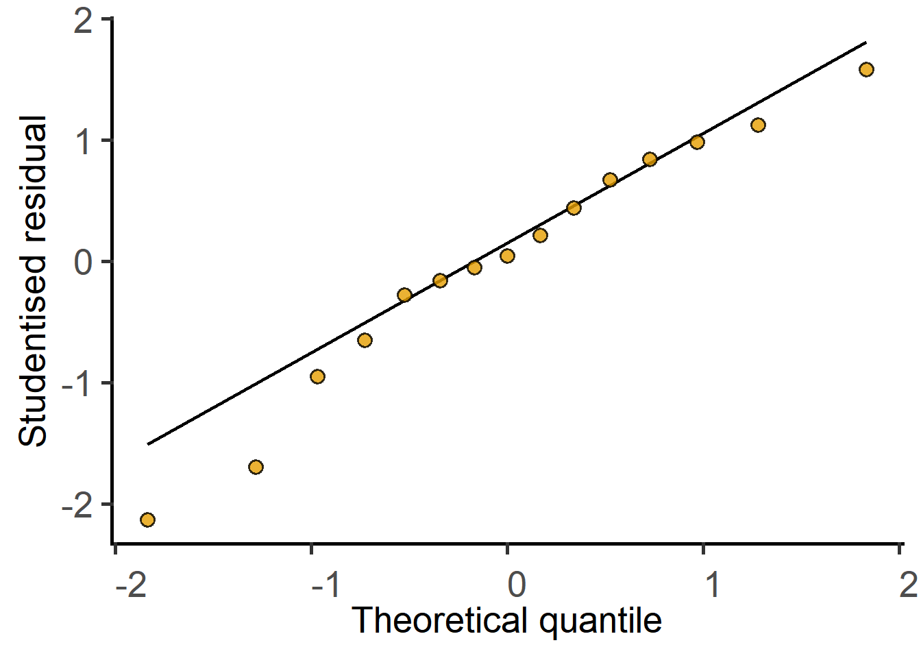
grafify#ANOVA table
mixed_anova(data = Bact,
Y_value = "logit(Death/100)",
Fixed_Factor = "Genotype",
Random_Factor = "Experiment")boundary (singular) fit: see help('isSingular')Type II Analysis of Variance Table with Kenward-Roger's method
Sum Sq Mean Sq NumDF DenDF F value Pr(>F)
Genotype 23.48 11.74 2 8 191.18 1.764e-07 ***
---
Signif. codes: 0 '***' 0.001 '**' 0.01 '*' 0.05 '.' 0.1 ' ' 1#post-hoc comparison to reference group
posthoc_vsRef(Model = graf_1w_model,
Fixed_Factor = "Genotype",
Ref_Level = 1)$emmeans
Genotype response SE df lower.CL upper.CL
WT 0.2413 0.02030 12 0.1999 0.2882
mfg 0.0194 0.00211 12 0.0153 0.0245
yfg 0.1954 0.01740 12 0.1602 0.2361
Degrees-of-freedom method: kenward-roger
Confidence level used: 0.95
Intervals are back-transformed from the logit scale
$contrasts
contrast odds.ratio SE df null t.ratio p.value
mfg / WT 0.0621 0.00974 8 1 -17.730 <.0001
yfg / WT 0.7634 0.12000 8 1 -1.723 0.1232
Degrees-of-freedom method: kenward-roger
P value adjustment: fdr method for 2 tests
Tests are performed on the log odds ratio scale